NumPy

Lecture 05

Dr. Colin Rundel

What is NumPy?

NumPy is the fundamental package for scientific computing in Python. It is a Python library that provides a multidimensional array object, various derived objects (such as masked arrays and matrices), and an assortment of routines for fast operations on arrays, including mathematical, logical, shape manipulation, sorting, selecting, I/O, discrete Fourier transforms, basic linear algebra, basic statistical operations, random simulation and much more.

import numpy as np
np.__version__

'2.2.2'

Arrays

In general NumPy arrays are constructed from sequences (e.g. lists), nesting as necessary for the number of desired dimensions.

np.array([1,2,3])

array([1, 2, 3])

np.array([[1,2],[3,4]])

array([[1, 2],
       [3, 4]])

np.array([[[1,2],[3,4]], [[5,6],[7,8]]])

array([[[1, 2],
        [3, 4]],

       [[5, 6],
        [7, 8]]])

np.array([1.0, 2.5, np.pi])

array([1.        , 2.5       , 3.14159265])

np.array([[True], [False]])

array([[ True],
       [False]])

np.array(["abc", "def"])

array(['abc', 'def'], dtype='<U3')

Some properties of NumPy arrays:

Arrays have a fixed size at creation
All data must be homogeneous (i.e. consistent type)
Built to support vectorized operations
Avoids copying whenever possible (inplace operations)

dtype

NumPy arrays all have the type() numpy.ndarray - specific type stored in the arrray is recorded as the array’s dtype. This is accessible via the .dtype attribute and can be set at creation using the dtype argument.

np.array([1,1]).dtype

dtype('int64')

np.array([1.1, 2.2]).dtype

dtype('float64')

np.array([True, False]).dtype

dtype('bool')

np.array([3.14159, 2.33333], dtype = np.double)

array([3.14159, 2.33333])

np.array([3.14159, 2.33333], dtype = np.float16)

array([3.14 , 2.334], dtype=float16)

np.array([1,2,3], dtype = np.uint8)

array([1, 2, 3], dtype=uint8)

dtypes and overflow

Some types have a maximum and or minimum value that can be stored in them. If you try to create an array with a value outside of this range you will get an overflow error. If you are instead coercing values using astype() you will not get this error.

np.array([-1, 1,2], dtype = np.uint8)

OverflowError: Python integer -1 out of bounds for uint8

np.array([1,2,1000], dtype = np.uint8)

OverflowError: Python integer 1000 out of bounds for uint8

np.array([-1, 1,2,1000]).astype(np.uint8)

array([255,   1,   2, 232], dtype=uint8)

Creating 1d arrays

Some common functions and methods for creating useful 1d arrays:

np.arange(10)

array([0, 1, 2, 3, 4, 5, 6, 7, 8, 9])

np.arange(3, 5, 0.25)

array([3.  , 3.25, 3.5 , 3.75, 4.  , 4.25, 4.5 , 4.75])

np.linspace(0, 1, 11)

array([0. , 0.1, 0.2, 0.3, 0.4, 0.5, 0.6, 0.7, 0.8, 0.9, 1. ])

np.logspace(0, 2, 4)

array([  1.        ,   4.64158883,  21.5443469 , 100.        ])

np.ones(4)

array([1., 1., 1., 1.])

np.zeros(6)

array([0., 0., 0., 0., 0., 0.])

np.full(3, False)

array([False, False, False])

np.empty(4)

array([1., 1., 1., 1.])

Creating 2d arrays (matrices)

Many of the same functions exist with some additional useful tools for common matrices,

np.eye(3)

array([[1., 0., 0.],
       [0., 1., 0.],
       [0., 0., 1.]])

np.identity(2)

array([[1., 0.],
       [0., 1.]])

np.zeros((2,2))

array([[0., 0.],
       [0., 0.]])

np.diag([3,2,1])

array([[3, 0, 0],
       [0, 2, 0],
       [0, 0, 1]])

np.tri(3)

array([[1., 0., 0.],
       [1., 1., 0.],
       [1., 1., 1.]])

np.triu(np.full((3,3),3))

array([[3, 3, 3],
       [0, 3, 3],
       [0, 0, 3]])

Creating \(n\)d arrays

For higher dimensional arrays just add dimensions when constructing,

np.zeros((2,3,2))

array([[[0., 0.],
        [0., 0.],
        [0., 0.]],

       [[0., 0.],
        [0., 0.],
        [0., 0.]]])

np.ones((2,3,2,2))

array([[[[1., 1.],
         [1., 1.]],

        [[1., 1.],
         [1., 1.]],

        [[1., 1.],
         [1., 1.]]],

       [[[1., 1.],
         [1., 1.]],

        [[1., 1.],
         [1., 1.]],

        [[1., 1.],
         [1., 1.]]]])

Subsetting

Arrays are subsetted using the standard python syntax with either indexes or slices, dimensions are separated by commas.

x = np.array([[1,2,3],[4,5,6],[7,8,9]])
x

array([[1, 2, 3],
       [4, 5, 6],
       [7, 8, 9]])

x[0]

array([1, 2, 3])

x[0,0]

np.int64(1)

x[0][0]

np.int64(1)

x[0:3:2, :]

array([[1, 2, 3],
       [7, 8, 9]])

x[0:3:2, :]

array([[1, 2, 3],
       [7, 8, 9]])

x[0:3:2, ]

array([[1, 2, 3],
       [7, 8, 9]])

x[1:, ::-1]

array([[6, 5, 4],
       [9, 8, 7]])

Views and copies

Basic subsetting of ndarray objects does not result in a new object, but instead a “view” of the original object. There are a couple of ways that we can investigate this behavior,

x = np.arange(10)
y = x[2:5]
z = x[2:5].copy()

f"{x=}, {x.base=}"

'x=array([0, 1, 2, 3, 4, 5, 6, 7, 8, 9]), x.base=None'

f"{y=}, {y.base=}"

'y=array([2, 3, 4]), y.base=array([0, 1, 2, 3, 4, 5, 6, 7, 8, 9])'

f"{z=}, {z.base=}"

'z=array([2, 3, 4]), z.base=None'

type(x), type(y), type(z)

(<class 'numpy.ndarray'>, <class 'numpy.ndarray'>, <class 'numpy.ndarray'>)

np.shares_memory(x,y)

True

np.shares_memory(x,z)

False

np.shares_memory(y,z)

False

y.flags

  C_CONTIGUOUS : True
  F_CONTIGUOUS : True
  OWNDATA : False
  WRITEABLE : True
  ALIGNED : True
  WRITEBACKIFCOPY : False

Subsetting with …

Unlike R, it is not possible to leave an argument blank - to select all elements with numpy we use :. To avoid having to type excess : you can use ... which expands to the number of : needed to account for all dimensions,

x = (np.arange(16)
     .reshape(2,2,2,2))
x

array([[[[ 0,  1],
         [ 2,  3]],

        [[ 4,  5],
         [ 6,  7]]],

       [[[ 8,  9],
         [10, 11]],

        [[12, 13],
         [14, 15]]]])

x[0, 1, :, :]

array([[4, 5],
       [6, 7]])

x[0, 1, ...]

array([[4, 5],
       [6, 7]])

x[:, :, :, 1]

array([[[ 1,  3],
        [ 5,  7]],

       [[ 9, 11],
        [13, 15]]])

x[..., 1]

array([[[ 1,  3],
        [ 5,  7]],

       [[ 9, 11],
        [13, 15]]])

Subsetting with tuples

Unlike lists, an ndarray can be subset by a tuple containing integers,

x = np.arange(6); x

array([0, 1, 2, 3, 4, 5])

x[(0,1,3),]

array([0, 1, 3])

x[(3,5,1,0),]

array([3, 5, 1, 0])

x[(0,1,3)]

IndexError: too many indices for array: array is 1-dimensional, but 3 were indexed

x = np.arange(16).reshape((4,4))
x

array([[ 0,  1,  2,  3],
       [ 4,  5,  6,  7],
       [ 8,  9, 10, 11],
       [12, 13, 14, 15]])

x[(0,1,3), :]

array([[ 0,  1,  2,  3],
       [ 4,  5,  6,  7],
       [12, 13, 14, 15]])

x[:, (0,1,3)]

array([[ 0,  1,  3],
       [ 4,  5,  7],
       [ 8,  9, 11],
       [12, 13, 15]])

x[(0,1,3), (0,1,3)]

array([ 0,  5, 15])

Subsetting assignment

Most of the subsetting approaches we’ve just seen can also be used for assignment, just keep in mind that we cannot change the size or type of the ndarray,

x = np.arange(9).reshape((3,3)); x

array([[0, 1, 2],
       [3, 4, 5],
       [6, 7, 8]])

x[0,0] = -1; x

array([[-1,  1,  2],
       [ 3,  4,  5],
       [ 6,  7,  8]])

x[0, :] = -2; x

array([[-2, -2, -2],
       [ 3,  4,  5],
       [ 6,  7,  8]])

x[0:2,1:3] = -3; x

array([[-2, -3, -3],
       [ 3, -3, -3],
       [ 6,  7,  8]])

x[(0,1,2), (0,1,2)] = -4; x

array([[-4, -3, -3],
       [ 3, -4, -3],
       [ 6,  7, -4]])

x [0,0] = "A"

ValueError: invalid literal for int() with base 10: 'A'

Reshaping arrays

The dimensions of an array can be retrieved via the shape attribute, these values can changed via the reshape() method or updating shape

x = np.arange(6); x

array([0, 1, 2, 3, 4, 5])

y = x.reshape((2,3)); y

array([[0, 1, 2],
       [3, 4, 5]])

np.shares_memory(x,y)

True

z = x
z.shape = (2,3)
z

array([[0, 1, 2],
       [3, 4, 5]])

array([[0, 1, 2],
       [3, 4, 5]])

np.shares_memory(x,z)

True

Implicit dimensions

When reshaping an array, the value -1 can be used to automatically calculate a dimension,

x = np.arange(6); x

array([0, 1, 2, 3, 4, 5])

x.reshape((2,-1))

array([[0, 1, 2],
       [3, 4, 5]])

x.reshape((-1,3,2))

array([[[0, 1],
        [2, 3],
        [4, 5]]])

x.reshape(-1)

array([0, 1, 2, 3, 4, 5])

x.reshape((-1,4))

ValueError: cannot reshape array of size 6 into shape (4)

Flattening arrays

We just saw one of the more common approaches to creating a flat view of an array (reshape(-1)), there are two other common methods / functions:

ravel creates a flattened view of the array and
flatten creates a flattened copy of the array.

w = np.arange(6).reshape((2,3)); w

array([[0, 1, 2],
       [3, 4, 5]])

x = w.reshape(-1)
x

array([0, 1, 2, 3, 4, 5])

np.shares_memory(w,x)

True

y = w.ravel()
y

array([0, 1, 2, 3, 4, 5])

np.shares_memory(w,y)

True

z = w.flatten()
z

array([0, 1, 2, 3, 4, 5])

np.shares_memory(w,z)

False

Resizing

The size of an array cannot be changed but a new array with a different size can be created from an existing array via the resize function and method. Note these have different behaviors around what values the new entries will have.

x = np.resize(
  np.ones((2,2)), 
  (3,3)
)
x

array([[1., 1., 1.],
       [1., 1., 1.],
       [1., 1., 1.]])

y = np.ones(
  (2,2)
).resize(
  (3,3)
)
y

Why didn’t this work?

y = np.ones(
  (2,2)
)
y.resize((3,3))
y

array([[1., 1., 1.],
       [1., 0., 0.],
       [0., 0., 0.]])

Joining arrays

concatenate() is a general purpose function for joining arrays, with specialized versions hstack(), vstack(), and dstack() for rows, columns, and slices respectively.

x = np.arange(4).reshape((2,2)); x

array([[0, 1],
       [2, 3]])

y = np.arange(4,8).reshape((2,2)); y

array([[4, 5],
       [6, 7]])

np.concatenate((x,y), axis=0)

array([[0, 1],
       [2, 3],
       [4, 5],
       [6, 7]])

np.concatenate((x,y), axis=1)

array([[0, 1, 4, 5],
       [2, 3, 6, 7]])

np.vstack((x,y))

array([[0, 1],
       [2, 3],
       [4, 5],
       [6, 7]])

np.hstack((x,y))

array([[0, 1, 4, 5],
       [2, 3, 6, 7]])

np.concatenate((x,y), axis=2)

numpy.exceptions.AxisError: axis 2 is out of bounds for array of dimension 2

np.concatenate((x,y), axis=None)

array([0, 1, 2, 3, 4, 5, 6, 7])

np.dstack((x,y))

array([[[0, 4],
        [1, 5]],

       [[2, 6],
        [3, 7]]])

NumPy numerics

Basic operators

All of the basic mathematical operators in Python are implemented for arrays, they are applied element-wise to the array values.

np.arange(3) + np.arange(3)

array([0, 2, 4])

np.arange(3) - np.arange(3)

array([0, 0, 0])

np.arange(3) + 2

array([2, 3, 4])

np.arange(3) * np.arange(3)

array([0, 1, 4])

np.arange(1,4) / np.arange(1,4)

array([1., 1., 1.])

np.arange(3) * 3

array([0, 3, 6])

np.full((2,2), 2) ** np.arange(4).reshape((2,2))

array([[1, 2],
       [4, 8]])

np.full((2,2), 2) ** np.arange(4)

ValueError: operands could not be broadcast together with shapes (2,2) (4,)

Mathematical functions

NumPy provides a wide variety of basic mathematical functions that are vectorized, in general they will be faster than their base equivalents (e.g. np.sum() vs sum()),

np.sum(np.arange(1000))

np.int64(499500)

np.cumsum(np.arange(10))

array([ 0,  1,  3,  6, 10, 15, 21, 28, 36, 45])

np.log10(np.arange(1,4))

array([0.        , 0.30103   , 0.47712125])

np.median(np.arange(10))

np.float64(4.5)

Matrix multiplication

is supported using the matmul() function or the @ operator,

x = np.arange(6).reshape(3,2)
y = np.tri(2,2)

x @ y

array([[1., 1.],
       [5., 3.],
       [9., 5.]])

y.T @ y

array([[2., 1.],
       [1., 1.]])

np.matmul(x.T, x)

array([[20, 26],
       [26, 35]])

y @ x

ValueError: matmul: Input operand 1 has a mismatch in its core dimension 0, with gufunc signature (n?,k),(k,m?)->(n?,m?) (size 3 is different from 2)

Other linear algebra functions

All of the other common linear algebra functions are (mostly) implemented in the linalg submodule.

np.linalg.det(y)

np.float64(1.0)

np.linalg.eig(x.T @ x)

EigResult(eigenvalues=array([ 0.43988174, 54.56011826]), eigenvectors=array([[-0.79911221, -0.6011819 ],
       [ 0.6011819 , -0.79911221]]))

np.linalg.inv(x.T @ x)

array([[ 1.45833333, -1.08333333],
       [-1.08333333,  0.83333333]])

np.linalg.cholesky(x.T @ x)

array([[4.47213595, 0.        ],
       [5.81377674, 1.09544512]])

Random values

NumPy has another submodule called random for functions used to generate random values.

In order to use this, you construct a generator via default_rng(), with or without a seed, and then use the generator’s methods to obtain your desired random values.

rng = np.random.default_rng(seed = 1234)

rng.random(3) # ~ Uniform [0,1)

array([0.97669977, 0.38019574, 0.92324623])

rng.normal(loc=0, scale=2, size = (2,2))

array([[ 0.30523839,  1.72748778],
       [ 5.82619845, -2.95764672]])

rng.binomial(n=5, p=0.5, size = 10)

array([2, 4, 2, 2, 3, 4, 4, 3, 3, 3])

Advanced Indexing

Advanced indexing is triggered when the selection object, obj, is a non-tuple sequence object, an ndarray (of data type integer or bool), or a tuple with at least one sequence object or ndarray (of data type integer or bool).

There are two types of advanced indexing: integer and Boolean.

Advanced indexing always returns a copy of the data (contrast with basic slicing that returns a view).

Integer array subsetting (lists)

Lists of integers can be used to subset in the same way:

x = np.arange(16).reshape((4,4)); x

array([[ 0,  1,  2,  3],
       [ 4,  5,  6,  7],
       [ 8,  9, 10, 11],
       [12, 13, 14, 15]])

x[[1,3]]

array([[ 4,  5,  6,  7],
       [12, 13, 14, 15]])

x[[1,3], ]

array([[ 4,  5,  6,  7],
       [12, 13, 14, 15]])

x[:, [1,3]]

array([[ 1,  3],
       [ 5,  7],
       [ 9, 11],
       [13, 15]])

x[[0,1,3],]

array([[ 0,  1,  2,  3],
       [ 4,  5,  6,  7],
       [12, 13, 14, 15]])

x[[0,1,3]]

array([[ 0,  1,  2,  3],
       [ 4,  5,  6,  7],
       [12, 13, 14, 15]])

x[[1.,3]]

IndexError: only integers, slices (`:`), ellipsis (`...`), numpy.newaxis (`None`) and integer or boolean arrays are valid indices

Integer array subsetting (ndarrays)

Similarly we can also us integer ndarrays:

x = np.arange(6)
y = np.array([0,1,3])
z = np.array([1., 3.])

x[y,]

array([0, 1, 3])

x[y]

array([0, 1, 3])

x[z]

IndexError: arrays used as indices must be of integer (or boolean) type

x = np.arange(16).reshape((4,4))
y = np.array([1,3])

x[y]

array([[ 4,  5,  6,  7],
       [12, 13, 14, 15]])

x[y, ]

array([[ 4,  5,  6,  7],
       [12, 13, 14, 15]])

x[:, y]

array([[ 1,  3],
       [ 5,  7],
       [ 9, 11],
       [13, 15]])

x[y, y]

array([ 5, 15])

Exercise 1

Given the following matrix,

x = np.arange(16).reshape((4,4))
x

array([[ 0,  1,  2,  3],
       [ 4,  5,  6,  7],
       [ 8,  9, 10, 11],
       [12, 13, 14, 15]])

write an expression to obtain the center 2x2 values (i.e. 5, 6, 9, 10 as a matrix).

Boolean indexing

Lists or ndarrays of boolean values can also be used to subset (positions with True are kept and False are discarded)

x = np.arange(6); x

array([0, 1, 2, 3, 4, 5])

x[[True, False, True, False, True, False]]

array([0, 2, 4])

x[[True]]

IndexError: boolean index did not match indexed array along axis 0; size of axis is 6 but size of corresponding boolean axis is 1

x[np.array([True, False, True, False, True, False])]

array([0, 2, 4])

x[np.array([True])]

IndexError: boolean index did not match indexed array along axis 0; size of axis is 6 but size of corresponding boolean axis is 1

Boolean expressions

The primary utility of boolean subsetting comes from vectorized comparison operations,

x = np.arange(6); x

array([0, 1, 2, 3, 4, 5])

x > 3

array([False, False, False, False,  True,  True])

x[x>3]

array([4, 5])

x % 2 == 1

array([False,  True, False,  True, False,  True])

x[x % 2 == 1]

array([1, 3, 5])

y = np.arange(9).reshape((3,3))
y % 2 == 0

array([[ True, False,  True],
       [False,  True, False],
       [ True, False,  True]])

y[y % 2 == 0]

array([0, 2, 4, 6, 8])

NumPy and Boolean operators

If we want to use a logical operators on an array we need to use &, |, and ~ instead of and, or, and not respectively.

x = np.arange(6); x

array([0, 1, 2, 3, 4, 5])

y = (x % 2 == 0); y

array([ True, False,  True, False,  True, False])

~y

array([False,  True, False,  True, False,  True])

y & (x > 3)

array([False, False, False, False,  True, False])

y | (x > 3)

array([ True, False,  True, False,  True,  True])

meshgrid()

One other useful function in NumPy is meshgrid() which generates all possible combinations between the input vectors (as a tuple of ndarrays),

pts = np.arange(3)
x, y = np.meshgrid(pts, pts)

array([[0, 1, 2],
       [0, 1, 2],
       [0, 1, 2]])

array([[0, 0, 0],
       [1, 1, 1],
       [2, 2, 2]])

np.sqrt(x**2 + y**2).round(3)

array([[0.   , 1.   , 2.   ],
       [1.   , 1.414, 2.236],
       [2.   , 2.236, 2.828]])

Exercise 2

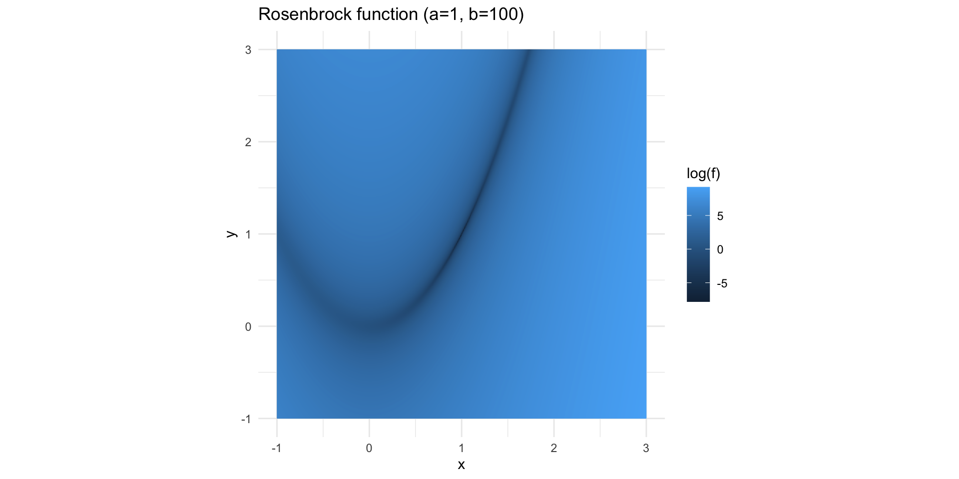
We will now use this to attempt a simple brute force approach to numerical optimization, define a grid of points using meshgrid() to approximate the minima the following function:

\[ f(x,y) = (1-x)^2 + 100(y-x^2)^2 \] Considering values of \(x,y \in (-1,3)\), which value(s) of \(x,y\) minimize this function?